Table of Contents
Introduction
In today’s world, who hasn’t used an LLM? LLMs are now used for a wide range of tasks, including translation, customer support, content generation, and contract review. As more people rely on LLMs, expectations for their performance continue to rise. For users, response time is one of the most important factors, as faster responses directly improve work efficiency.
In LLMs, one metric closely related to the user experience is KV cache. KV cache has evolved from being introduced as a basic optimization to becoming an area of active optimization through various techniques. Improving KV cache efficiency is becoming an important focus for the future development of LLM inference.
What Is KV Cache
When an LLM processes a request, such as when you enter a prompt and an AI generates a response token by token, the inference process can be broadly divided into two stages:
- Prefill (input processing stage) The model processes the entire input prompt at once. Since it is processing the input for the first time, it computes and generates intermediate data that will be reused throughout the subsequent generation process. This data is stored as the KV Cache. The computation in this stage can be substantial. It is similar to quickly reading through a book and taking notes on the information that may be needed later.
- Decode (generation stage) The model uses this cached data to generate the response one token at a time. When generating a new token, the model does not need to process the entire input again. Instead, it reads the relevant information from the KV Cache and uses it to generate the next token. The KV Cache is then updated with the K and V values of the newly generated token. Each individual decode step requires less computation than prefill, but it repeatedly reads and writes the KV Cache. This makes decode performance highly sensitive to GPU memory bandwidth.
The KV Cache serves as an essential bridge between these two stages. KV Cache stands for Key-Value Cache. More precisely, it stores the intermediate attention-state data generated during LLM inference, specifically the Key (K) and Value (V) tensors produced by the attention mechanism. By reusing these tensors during decoding, the model avoids recomputing the attention states of previously processed tokens.
Why Was KV Cache Introduced?
To understand why KV Cache was introduced, we first need to look at the autoregressive mechanism used by large language models.
When generating a response, an LLM typically uses an autoregressive approach. In simple terms, the model does not generate the entire response at once. Instead, it generates one token at a time. For example, the model first generates Token A based on the user input. It then adds A to the existing context and generates Token B based on the user input and Token A. The model then uses the updated context to generate Token C, and continues this process. During attention computation, each token produces three tensors: Query (Q), Key (K), and Value (V).
However, autoregressive generation introduces an efficiency problem. When generating Token C, the K and V values of Tokens A and B would otherwise need to be computed again. The Query values are not reused in subsequent steps. This means that each new token can trigger repeated computation of the K and V values for an increasingly large number of historical tokens. As the sequence grows, these repeated computations increase both the computational overhead and inference latency.
In 2017, the Google team published Attention Is All You Need, which introduced the Transformer architecture and the Query, Key, and Value mechanism used in Attention. The architecture also uses the Decoder for autoregressive generation. During token-by-token decoding, the K and V values of previously processed tokens do not change. They can therefore be stored and reused in subsequent decoding steps. This property provides the technical basis for implementing KV Cache. KV Cache can therefore be understood as a natural inference optimization for autoregressive decoding in Transformer-based models. It has since become a widely used inference optimization in Transformer-based generative LLMs, including GPT, Llama, and Qwen.
KV Cache does not change how an LLM generates a response autoregressively, one token at a time. Instead, it caches the K and V values of historical tokens to avoid redundant computation. It trades additional GPU memory usage for higher inference efficiency.
As long-context workloads, multi-turn conversations, and high-concurrency LLM services become more common, KV Cache consumes an increasing amount of GPU memory. It has also become an important factor affecting LLM inference latency, throughput, and GPU memory management.
Modern LLM inference is typically divided into the Prefill and autoregressive Decode stages, with the KV Cache continuously read and extended during the Decode stage.
For an introduction to P-D disaggregation, see: What is Prefill-Decode Disaggregation and How to Cut CAPEX for AI Inference Fabrics by Around 30%.
How Does KV Cache Work?
Now that we understand why KV Cache is needed, let’s look at how it works. The overall process can be divided into two stages: Prefill and Decode.
Prefill: Compute and Store the KV Cache
After the user enters a Prompt, the model first enters the Prefill stage.
For example, if the user input contains 1,000 tokens, the model processes all 1,000 tokens in parallel. It computes the corresponding Key and Value tensors across the Transformer layers and stores them in the KV Cache in GPU memory. These cached K and V tensors serve as reusable attention states for subsequent decoding.
The core tasks of this stage are to process the complete Prompt, build the initial KV Cache, and predict the first output token.
Decode: Read and Extend the KV Cache
After Prefill is complete, the model starts generating the response one token at a time. This is the Decode stage.
For example, when generating the 1,001st token, the model reads the cached K and V values of the previous 1,000 tokens. At the same time, it computes the Q, K, and V values for the new token. After the Attention computation, the model generates the new token and appends its K and V values to the KV Cache.
When generating the 1,002nd token, the model reads the existing KV Cache again and appends the K and V values of the 1,002nd token. This process continues with each newly generated token.
Therefore, the KV Cache can be simply understood as a continuously growing storage area for historical K/V values:
Prefill
1,000 Tokens
↓
Compute K/V
↓
┌─────────────────────┐
│ K1 K2 … K1000 │
│ V1 V2 … V1000 │
└─────────────────────┘
KV Cache
Decode
Generate Token 1001
↓
Read historical K/V + compute Q/K/V for the new token
↓
Append K1001 / V1001
Generate Token 1002
↓
Read historical K/V + compute Q/K/V for the new token
↓
Append K1002 / V1002
To make the roles of K and V easier to understand, we can extend the “notes” analogy:
- K tensor (Key): Think of K as the “keywords” or “index” in a set of notes. When the model generates the next token, it compares the current state with all K values to determine which historical information is most relevant.
- V tensor (Value): Think of V as the “detailed information” associated with each index entry. Once the model identifies the relevant historical information through K, it retrieves the corresponding information from V and uses it to compute the output token.
This process shows that the KV Cache is essentially a classic space-for-time trade-off. It uses additional GPU memory to store the historical K and V values that have already been computed. When generating subsequent tokens, the model can reuse these cached states instead of recomputing them, reducing redundant computation and improving inference efficiency.
KV Cache Is Growing Rapidly
Enterprise GPU servers are handling more concurrent conversations, while the supported context length of each conversation continues to increase. Let’s run the numbers.
Assume your service has 100 concurrent users sending requests at the same time, and each user provides a long context of 32K (32,000) tokens:
- KV Cache per user: 0.32 MB×32,000≈10 GB
- Total KV Cache for 100 concurrent users: 10 GB×100=1000 GB≈1 TB!
A high-end H100 GPU provides only 80 GB of GPU memory. A 1 TB KV Cache means that even if you do not need additional GPUs for compute capacity, you still need more GPUs simply to provide enough memory to hold the cache. This can require more than a dozen expensive GPUs.
This creates a significant burden for enterprises. However, the impact of growing KV Cache goes beyond GPU memory capacity.
As P-D disaggregation (decoupling the Prefill and Decode stages) becomes more common in modern AI infrastructure, KV Cache is shifting from static memory within a single GPU to massive volumes of East-West traffic exchanged frequently across nodes and racks.
After the Prefill nodes compute and partition the KV Cache for a long context, several gigabytes to tens of gigabytes of tensors must be transferred to Decode nodes within a very tight time window. This creates two major challenges for the data center network:
- Uncontrolled network infrastructure scaling: Operators may need to deploy high-end network infrastructure, including expensive 800G/1.6T optical transceivers, non-blocking Spine-Leaf topologies, and lossless networks based on RoCEv2 or InfiniBand. Network infrastructure costs can increase significantly as a result.
- Communication challenges with Context Parallelism (CP): When processing sequences with hundreds of thousands of tokens, Context Parallelism within Prefill nodes can trigger highly intensive All-to-All and All-Gather collective communication. Network congestion, packet loss, or PFC deadlocks can cause communication latency to offset the acceleration gained from compute resources. This makes network engineering a critical challenge for large-scale LLM inference.
What Can the Network Do as KV Cache Grows?
As KV Cache continues to grow and PD disaggregation introduces increasing cross-node traffic, traditional AI data centers often use RoFT (Rail-Optimized Fat-Tree) or standard Clos topologies. However, the bursty and uneven traffic patterns of KV Cache transfers can create localized hotspots on leaf links. Local link overload can keep switch egress queues at high occupancy for extended periods, frequently triggering PFC (Priority-based Flow Control) pause frames. This can cause congestion to propagate through the network and directly degrade the P99 tail latency of TTFT.
To address the bottlenecks of cross-node KV Cache transfers, next-generation inference network architectures, mainly address three areas at the architectural level:
- Topology Flattening (De-Spine Architecture)
This approach removes the Spine layer from the traditional multi-tier Clos architecture and builds a fully flattened interconnect for GPU servers. For example, Leaf switches can be divided into two groups and interconnected as a complete bipartite graph, limiting data transmission between any two GPU nodes to 2 switch hops. This shortens communication paths and reduces latency. It also significantly reduces the probability of congestion caused by multi-tier forwarding.
- Hybrid Single-Rail/Multi-Rail Connectivity and Network-Wide Path Distribution
The network uses a combination of single-rail and multi-rail connectivity. Multiple GPU NIC ports are connected to different switch groups. Combined with routing strategies optimized for the flattened topology, the network does not rely solely on simple hash-based path selection. Instead, bursty KV Cache traffic can be distributed across a broader set of non-conflicting paths. This helps eliminate avoidable congestion caused by uneven topology-to-traffic mapping at the architectural level.
- Hardware Right-Sizing for Lower Cost and Higher Performance
When congestion is prevented at the topology level, the cluster no longer needs to rely on excessive over-provisioning to compensate for local network bottlenecks.
- Lower CAPEX: For the same GPU scale, switch and high-density optical transceiver costs can be reduced by approximately 33%.
- Higher inference performance: By reducing PFC backpressure and queue buildup, effective network utilization can increase significantly. TTFT P99 tail latency can be reduced by more than 40%, while average GPU inference throughput can increase by more than 15%.
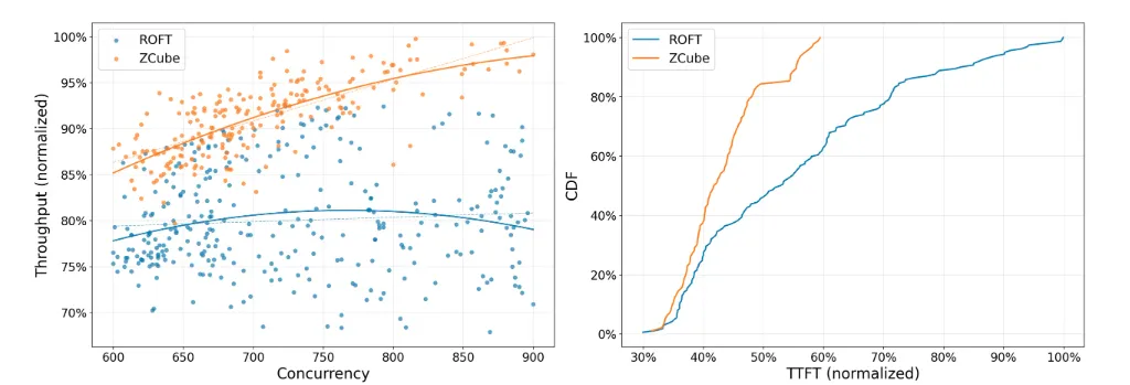
Asterfusion’s Architecture to Save CAPEX
Asterfusion has designed an architecture for P-D disaggregated inference scenarios. Compared with different network architectures, the solution reduces overall hardware costs by 26%–40%. The savings come not only from reducing the number of switches, but also from reducing the number of optical transceivers required.
Stay tuned for more details.


