How to Read NCCL Test Results and What Really Matters for AI Clusters

I. AI scale expansion is shifting the bottleneck: from compute to communication

As large-scale model training and AI inference continue to grow, the bottleneck in GPU clusters is undergoing a fundamental shift: in the past, performance was primarily constrained by compute power, but increasingly it is being limited by “communication.” In other words, the issue is no longer that GPUs are not fast enough, but that data movement between GPUs is not fast enough. Against this backdrop, NCCL (NVIDIA Collective Communications Library) and its benchmarking tools have become important instruments for evaluating AI cluster performance.

However, in practice, NCCL test reports commonly suffer from three issues:

• Metrics are complex and terminology-heavy, making them difficult to interpret
• Analysis is GPU-centric and often overlooks the network layer
• Test environments are overly idealized and deviate from real-world production conditions

As a result, NCCL outputs often lead to a situation where “data is visible, but conclusions are not.”

II. What exactly is NCCL test?

“NCCL is not a tool that measures GPUs or networks separately. Instead, it is a system-level indicator of how well the network can support GPU collaboration as the system scales up.” In other words, NCCL is not a single benchmark, but a three-layer mapping:

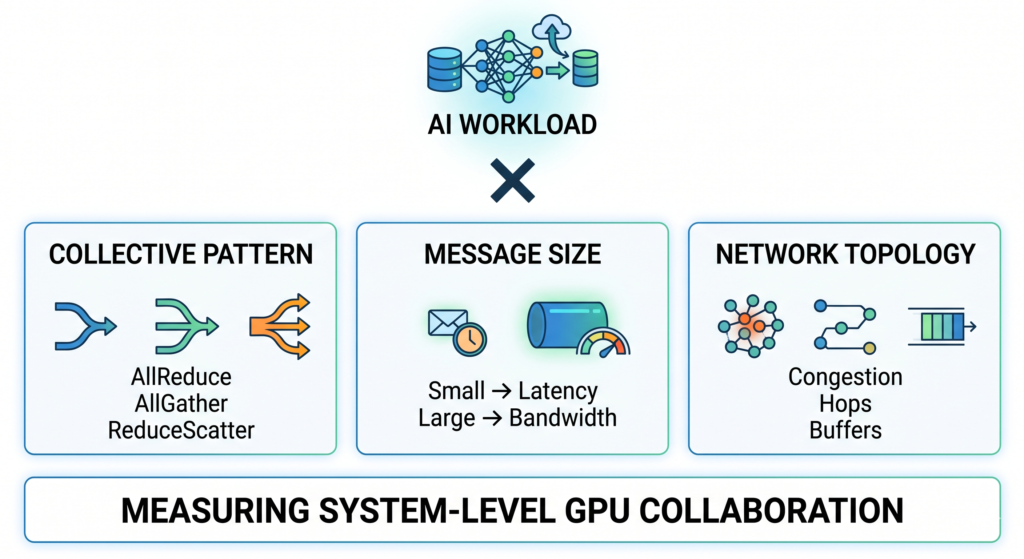
Collective Pattern (communication patterns)

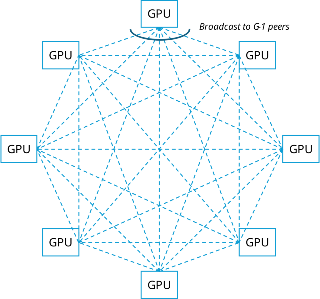
• AllReduce (gradient synchronization)
• AllGather (parameter collection)
• ReduceScatter (distributed computation partitioning)

Message sizes

At the same time, different message sizes trigger completely different network behaviors:

• Small messages → latency-bound
• Large messages → bandwidth-bound

Topology Interaction (network behavior)

• Congestion
• Hop count
• Buffer behavior

In other words, NCCL can be understood as a combined evaluation of: communication pattern × message size × network topology. But on top of these three layers, there is an even more important upper-level variable: the AI workload itself.

Different AI Workloads Lead to Completely Different NCCL Behaviors

In real-world AI clusters, one critical but often overlooked point is that NCCL benchmark results must be interpreted in the context of the specific AI training paradigm. Otherwise, it is very easy to draw misleading conclusions. Different parallelism strategies fundamentally determine communication patterns, which in turn directly shape NCCL performance:

Data Parallelism

• Core communication: AllReduce
• Characteristics: global synchronization is required in every training step

Network requirements: Low latency (determines per-step training time) and high stability (to avoid slowdowns caused by stragglers or waiting nodes)

Tensor Parallelism

• Core communication: AllReduce + AllGather
• Characteristics: frequent communication with larger data volume

Network requirements: High bandwidth efficiency and strong congestion control capability

Pipeline Parallelism

• Core communication: point-to-point (P2P) communication

Network requirements: High stability (low jitter is critical) and predictable latency

Different AI workloads essentially define what the NCCL performance curve should look like. If NCCL results are interpreted without considering the workload context, the conclusions are likely to be misleading or even meaningless.

Workload	NCCL Pattern	Network Requirement
Data Parallel	AllReduce	Low latency + high bandwidth
Tensor Parallel	AllReduce + AllGather	High bandwidth
Pipeline	P2P	Stability

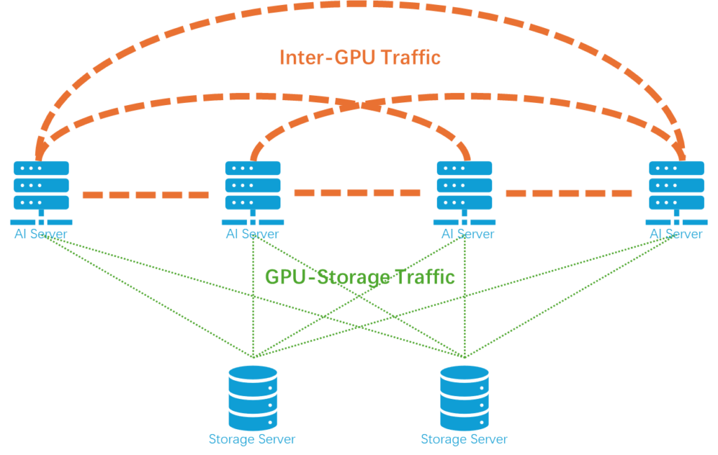
For more about GPU interconnect :Unveiling AI Data Center Network Traffic

III. How to Decompose NCCL Results: GPU-side vs Network-side

NCCL outputs an end-to-end result is as below:

GPU → PCIe / NVLink → NIC → Network → NIC → PCIe / NVLink → GPU

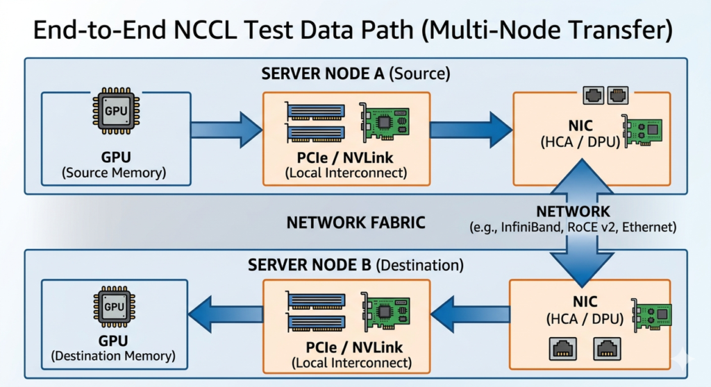
However, it does not explicitly indicate where the bottleneck occurs. From an engineering perspective, it can be clearly decomposed into two parts:

GPU-side Metrics

Key characteristics: most impactful in small-scale tests, factors originating from GPU computation and intra-node interconnects such as PCIe/NVLink.

Metric	Description	Desired Direction
Small message throughput	Performance of small-size communication (GPU kernel + PCIe/NVLink)	Higher is better
Intra-node performance	Communication efficiency within a single node	Higher is better
NCCL algorithm efficiency	Efficiency of NCCL algorithms (Ring / Tree / NVLS, etc.)	Higher is better
GPU utilization	How effectively GPUs are being utilized during communication	Higher is better
NVLink / PCIe bandwidth	Local interconnect bandwidth between GPUs	Higher is better

Network-side Metrics

Key characteristics: determine the upper limit in large-scale clusters, performance constraints introduced by the network fabric, including bandwidth, latency, congestion, and topology effects.

Metric	Description	Desired Direction
Large message bandwidth	Throughput under large-scale communication (closer to real training)	Higher is better
AllReduce time	Time required to complete synchronization	Lower is better
P95 / P99 latency	Tail latency (network stability under load)	Lower is better
Packet loss / retransmission	Packet loss and retransmission rate	Lower is better
Flow imbalance	Degree of traffic imbalance across paths	Lower is better
Scale-out efficiency	Performance retention when scaling to larger cluster sizes	Higher is better

IV. Key Insight: NCCL Performance Changes with Scale — Essentially a “Bottleneck Migration”

The most important value of NCCL benchmarking is not a single number, but a trend: as scale increases, the bottleneck gradually shifts from GPU to the network. At small scale, it is a GPU problem; at large scale, it becomes a network problem.

4.1 Small Scale Stage: GPU-Dominated (1–4 Nodes)

At small scale, computation is mainly concentrated within a single node or a very small number of nodes. At this stage, performance bottlenecks are almost entirely driven by the GPU itself rather than the network. This phase can be understood as pushing single-node performance to its limit.

Within the range of 1 to 4 nodes, much of the communication happens inside the same chassis, where GPUs exchange data via NVLink or PCIe. The bandwidth and topology of these local interconnects directly determine whether GPUs can collaborate efficiently. For example, in systems with H100 GPUs, NVLink provides extremely high bandwidth, and any issue here will significantly reduce GPU utilization (MFU).

At this stage, NCCL communication algorithms (such as Ring or Tree) are primarily optimized for efficient data movement within memory and interconnects, rather than cross-network communication. Therefore, the key focus here is whether the GPU itself is “healthy.”

• Key observation: Check whether the GPU is “healthy”
• Metrics of interest: compute utilization, memory bandwidth utilization, per-GPU temperature and power (thermal throttling)
• Pain point: a single GPU failure or unstable PCIe link can stall the entire job

4.2 Medium Scale Stage: GPU + Network Hybrid (8–32 Nodes)

When the scale grows to 8–32 nodes, the system crosses the “single-machine boundary,” and the network starts to actively participate and significantly influence performance.

At this stage, GPU-to-GPU communication is no longer confined within a single node but increasingly happens across nodes. Even if single-node compute power is strong, insufficient network latency or bandwidth can noticeably slow down overall training. In this sense, compute begins to be “diluted” by the network.

To reduce latency and CPU overhead, technologies such as RDMA and RoCE v2 are typically introduced to enable direct remote memory access. However, this also makes network configuration far more critical. Improper tuning of lossless networking mechanisms such as PFC and ECN can easily lead to performance degradation.

In addition, multi-tier switching topologies (e.g., Spine-Leaf) begin to appear at this stage, making whether the network is truly non-blocking critically important. Even slight oversubscription can introduce latency variability.

• Key observation: Check whether the system is “balanced”
• Metrics of interest: communication-to-computation overlap ratio, network P99 latency, switch buffer occupancy
• Pain point: the “weakest link effect” emerges — even a single retransmission event on one port can slow down the entire 32-node group

4.3 Large Scale Stage: Network-Dominated (64+ Nodes)

When the system scales to 64 nodes, or even hundreds or thousands of nodes, the network is no longer a supporting component — it becomes the core infrastructure that determines the upper limit of AI cluster performance.

At this stage, the network effectively becomes the computer itself. While GPU performance still matters, the actual training efficiency is primarily determined by network topology, traffic scheduling, and overall communication strategy.

For example, large-scale deployments typically adopt Leaf-Spine or multi-tier Clos architectures. The design of these topologies directly impacts communication path length and bandwidth utilization. To reduce cross-switch traffic, designs such as rail-optimized placement are often used, ensuring GPUs with similar indices across nodes are connected to the same switch layer to improve parallel efficiency.

In addition, in high-speed 400G or 800G networks, stability requirements become extremely strict. Even a very small packet loss rate (e.g., 0.1%) can trigger retransmissions and significantly degrade NCCL performance. As a result, load balancing, congestion control, and adaptive routing become mandatory capabilities.

The key question at this stage is whether the system can continue to scale. This can be evaluated using speedup curves, scalability trends, and overall job completion time. If performance shows a clear inflection point as node count increases, it indicates that the network has become the bottleneck.

• Key observation: Check whether the system can still “scale”
• Metrics of interest: linear speedup factor, checkpointing overhead, mean time between failures (MTBF)
• Pain point: the operational burden shifts from GPUs to optical modules, fiber links, and switch configuration, especially in Fat-Tree topologies where physical cabling complexity becomes significant

V. Why NCCL Is Often Misinterpreted

The main reason NCCL is frequently misinterpreted is simple: many people treat observed metrics as conclusions rather than signals of underlying behavior.

For example:

• Bandwidth ≠ actual network capability
• Latency ≠ end-to-end performance
• Average values ≠ real-world experience

NCCL only tells you “what happened”, but it does not explain “why it happened.”

VI. How to Correctly Interpret NCCL: Identifying Network Bottlenecks from End-to-End Metrics

6.1 Message Size Distribution: The Foundation of Performance Curves

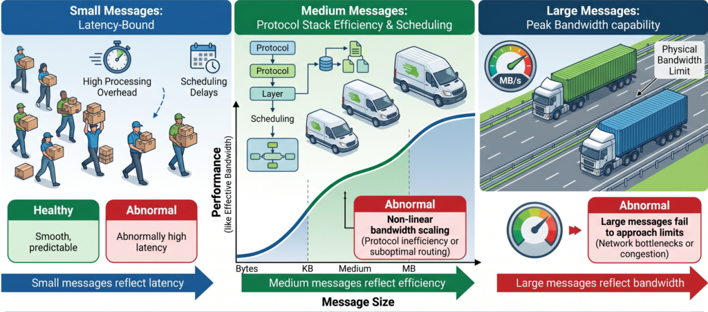
Message Size distribution is the starting point for understanding NCCL behavior. It represents the amount of data transferred in each communication operation, typically measured in bytes, KB, or MB. Although it seems simple, it has a major impact on network behavior. You can think of it as a logistics analogy: whether you are transporting small packages or an entire truckload of goods.

Different “shipment sizes” impose completely different requirements on the network. In NCCL, different message sizes correspond to different bottlenecks:

• Small messages are latency-bound
• Medium messages are limited by protocol stack efficiency and scheduling
• Large messages stress the peak bandwidth capability of the network

Beyond this, it is more important to observe the continuity and stability across the full message range, which reflects whether the network is healthy.

A healthy system typically shows:

• Smooth performance transition across small, medium, and large messages
• A continuous curve without sharp discontinuities
• Behavior that matches expectations (latency → protocol → bandwidth scaling progressively)

Abnormal patterns usually include:

• Abnormally high latency for small messages → excessive control-plane or scheduling overhead
• Non-linear bandwidth scaling for medium messages → protocol inefficiency or suboptimal routing
• Large messages failing to approach physical bandwidth limits → network bottlenecks or congestion

In summary: small messages reflect latency, medium messages reflect efficiency, and large messages reflect bandwidth. The continuity of the overall curve determines system health.

6.2 Latency Metrics: Focus on P95 and P99 Tail Latency

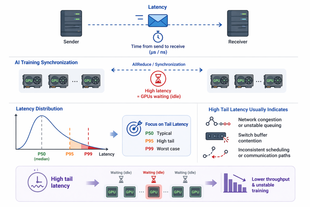
Latency refers to the time required for a communication operation from initiation to completion, typically measured in microseconds (μs) or even nanoseconds (ns). In simple terms, it answers: how long does it take for a message to reach the receiver after being sent?

In AI training, almost every step requires synchronization between nodes (e.g., AllReduce). If communication latency is high, GPUs must wait, leading to idle time and directly slowing down overall training throughput. More importantly, performance is not determined by average latency, but by the slowest portion — the tail latency. Therefore, in practice, beyond P50 (median), engineers should focus on P95 and P99, which reflect worst-case behavior. Optimizing AI networks is largely about reducing this tail latency.

If tail latency fluctuates significantly, it usually indicates:

• Network congestion or unstable queuing
• Switch buffer contention
• Inconsistent scheduling or communication paths

These issues directly impact the stability of training step time.

6.3 Bandwidth Metrics (Bus vs Algorithm Bandwidth)

NCCL typically provides two types of bandwidth metrics:

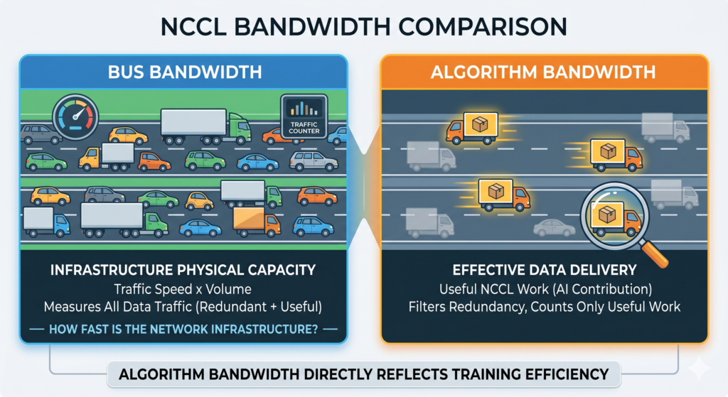
Bus Bandwidth represents the actual throughput of data transfer across GPUs, NICs, and switches. You can think of it as the overall capacity of a highway system — the product of traffic speed and traffic volume, reflecting how much data is physically moving across the network. It answers the question: how fast is the network infrastructure itself?

Algorithm Bandwidth is more “intelligent.” It measures the effective data transfer rate that actually contributes to the NCCL algorithm (e.g., AllReduce). In real execution, data may traverse multiple hops or be transferred multiple times (e.g., in ring-based AllReduce). As a result, Bus Bandwidth may appear high, but part of it includes redundant or repeated transfers.

Algorithm Bandwidth filters out this overhead and only counts useful data movement. In other words, not all traffic on the road is delivering goods — some is just circulation or rerouting. Algorithm Bandwidth only measures the vehicles that actually complete delivery.

Therefore, Algorithm Bandwidth is generally more meaningful in AI training scenarios because it directly reflects training efficiency.

6.4 Scaling Efficiency: The Key Metric for AI Cluster Scalability

In large model training, AllReduce is the core communication operation, determining how efficiently all GPUs synchronize gradients. However, cluster capability cannot be evaluated based only on single-node performance (8 or 16 GPUs), since single-node performance is usually close to ideal due to NVLink or intra-node interconnects.

What truly defines system scalability is the scaling curve, i.e., how communication performance evolves as GPU count increases.

(1) Small Scale: Validating Basic Health

At 8–16 GPUs, the focus is on whether the basic communication path is healthy:

• Whether bandwidth is fully utilized
• Whether NCCL communication paths are correct
• Whether intra-node interconnects are functioning properly

If performance is already abnormal at this stage, the issue lies in the infrastructure, not scaling.

(2) Medium Scale: Checking Whether Degradation Is Controlled

As the system scales from 8 → 32 → 64 GPUs, performance degradation is expected. The key question is not whether it drops, but whether it drops smoothly.

If the decline is continuous and predictable, the network is still healthy.

If the drop is sharp or irregular, it usually indicates:

• Multi-node communication constraints
• Bandwidth bottlenecks in Spine-Leaf architecture
• Insufficient congestion control or traffic scheduling

(3) Large Scale: Identifying the Inflection Point

When scaling further (64 → 128 → 256 GPUs), a sudden performance drop or inability to scale indicates a critical inflection point.

This typically means:

• Uplink bandwidth has become the bottleneck
• Network topology can no longer support current communication patterns
• Cross-switch communication efficiency has degraded significantly

In essence, the system transitions from “scalable” to “scaling-limited.” The scaling curve answers a fundamental question: Can the AI system maintain efficient communication as GPU count increases? It is not about speed, but about scalability.

6.5 Jitter: A Hidden Metric More Important Than Averages

Jitter refers to instability in packet arrival times. In ideal NCCL communication, messages should be transmitted at a steady rhythm. However, in Spine-Leaf networks, this stability is often disrupted.

Main causes include:

• ECMP hash collisions leading to uneven link utilization
• Microbursts in AI traffic saturating switch buffers
• Retransmissions caused by small packet loss events

Jitter is critical because NCCL AllReduce is a fully synchronized operation: all GPUs must complete communication before proceeding to the next step. If even a small number of GPUs are delayed, the entire cluster is slowed down — a classic “weakest link effect.”

For example, in a 1024-GPU cluster, even if 99.9% of GPUs complete in 2μs, a very small fraction experiencing 2ms jitter will increase the overall step time to 2ms. This is a clear case where local anomalies degrade global performance, which cannot be captured by averages.

Therefore, NCCL analysis must focus on P99 latency and variance. Frequent spikes or instability usually indicate:

• Microbursts in the network
• Congestion issues
• Scheduling jitter

These issues do not affect peak bandwidth but significantly reduce training efficiency and destabilize step time.

Note: When interpreting above NCCL metrics, a very common misunderstanding is to categorize them simply as “network metrics.” In reality, all of these metrics are derived from end-to-end measurements. This means the data reflects the entire communication path: GPU → NVLink / PCIe → NIC → Network → NIC → GPU

NCCL does not explicitly distinguish between a “GPU issue” and a “network issue”; it only reports the final observed behavior. However, in engineering practice, one key insight still holds: as scale increases, the dominant factor behind these metrics gradually shifts from the GPU side to the network side.

Therefore:

• At small scale, these metrics mainly reflect GPU and local interconnect performance
• At medium-to-large scale, they increasingly reflect network behavior
• At very large scale, they can almost be treated as “network capability indicators”

Although these metrics are commonly used to evaluate network performance, they are fundamentally end-to-end results. The only reason they are often interpreted as network metrics is that, at larger scale, the network becomes the dominant factor in the overall communication path.

VII. How to Determine if a Network Is Suitable for AI: Four Key Criteria

Evaluating the quality of an AI network should not be based solely on peak bandwidth. Instead, it must be assessed in the context of real training workloads. The core evaluation can be summarized into four key criteria:

7.1 Whether Bandwidth Utilization Approaches Physical Limits

Bandwidth is not equal to actual performance. In real AI clusters, the bottleneck is no longer simply “whether bandwidth exists,” but whether it can be efficiently utilized. In a typical Spine-Leaf architecture, can the network consistently maintain over 95% link utilization at scale? If performance drops significantly as the cluster expands, it usually indicates issues in load balancing or traffic routing.

7.2 Whether Tail Latency Is Controllable

Beyond average values, P95 and P99 latency are far more important indicators of real performance. A well-designed network should exhibit a highly stable tail latency distribution, ensuring that most communications complete within a consistent time window, thereby minimizing GPU idle time.

7.3 Small Message Performance Is the Key to Training Efficiency

In AI training, a large portion of communication is not large data transfers, but frequent gradient synchronization operations (e.g., AllReduce). NCCL benchmark results show that latency and small-packet handling capability often have a more direct impact on training step time than peak bandwidth.

This leads to an important conclusion: AI training is not file transfer — it is high-frequency, small-data, tightly synchronized communication.

7.4 Whether the Scaling Curve Is Smooth

When scaling from small clusters (e.g., 8 nodes) to large clusters (e.g., 256 nodes), does performance remain approximately linear?

If there is a noticeable inflection point or degradation during scaling, it indicates that the architecture cannot sustain large-scale AI training efficiently.

7.5 Stability Under Oversubscription and Traffic Bursts

In high-load or oversubscribed scenarios (e.g., 1:0.75 or 1:0.5), can the network still maintain near-theoretical performance?

This directly reflects the network’s resilience and stability under AI traffic characteristics such as microbursts and sudden communication spikes.

IX. NCCL Test Report Reading Playbook

This article is more hands-on. It provides a practical, “ready-to-use” guide for quickly interpreting NCCL test reports. Overall, this article is focused on actionable methodology. It minimizes conceptual explanations and emphasizes direct application and practical interpretation. For more: NCCL Test Report Reading Playbook.

Asterfusion 800G Test White Paper: Defining “High-Performance AI Networking” with Data

To validate the real-world performance of 800G high-performance Ethernet, Asterfusion conducted in-depth NCCL benchmarking based on the CX864E-N switch. Below are several key findings from the report that have the potential to redefine industry standards:

• Breakthrough in Nanosecond-Level Latency
  In a full Spine-Leaf topology, the end-to-end latency is only 2 μs, fully meeting and even exceeding UEC requirements. At the single-switch level, latency is as low as 560 ns. This means that during synchronization of tens of millions of parameters, network-induced stalls are reduced to the physical limit of microseconds—effectively eliminating GPU idle time caused by slow network response.
• The Power of Adaptive Routing (IAR)
  Eliminating the “network tax” and reclaiming 13% of lost bandwidth. To address the long-standing issue of hash collisions in Ethernet, Asterfusion introduced INT-Driven Adaptive Routing (IAR). Test results show that traditional ECMP hashing achieves only 84.57% bandwidth utilization in a Spine-Leaf architecture. With IAR enabled, utilization increases dramatically to 97%. This additional 13% directly translates into shorter training time and higher ROI on compute resources.
• Eliminating Tail Latency, Improving JCT
  Compared to traditional ECMP 5-tuple hashing, Asterfusion’s IAR reduces P95 Flow Completion Time (FCT) by 11.13%. This improvement directly boosts training efficiency. For example, in a typical LLaMA model training scenario, overall Job Completion Time (JCT) is reduced by approximately 6.12%.
• High Reliability Under Extreme Pressure
  Even under an oversubscription ratio of 1:0.5, the network achieves 96.88% of theoretical maximum completion. This demonstrates that, even under highly constrained resources, the congestion control and scheduling mechanisms can fully utilize every bit of available bandwidth. Such strong congestion management capabilities (PFC + ECN) are critical to ensuring lossless and retransmission-free operation in large-scale GPU clusters under bursty traffic conditions.

If all you need is a wider pipe, upgrading from 400G to 800G will get you there. But if what you want is faster model iteration cycles (JCT), you need a network that delivers 97% bandwidth utilization and reduces training time by 6.12%—like the Asterfusion CX864E-N 800G solution.

Conclusion

NCCL benchmarks are not just numbers. They are a window into how your network behaves under real AI workloads. Understanding them correctly means understanding your bottlenecks—not just your bandwidth. As AI continues to scale, the gap between a “working” network and a “high-performance” network becomes critical. And in that gap, it is network design—not just speed—that will define the winners.

Reference:

https://developer.nvidia.com/nccl

github.com/NVIDIA/nccl-tests

Unveiling AI Data Center Network Traffic – Asterfusion Data Technologies

Boost NCCL Cluster Performance With INT-Based Routing