Table of Contents
With the rise of large language models (LLMs), data centers are undergoing unprecedented changes. The scale of AI models is enormous and continues to grow rapidly. The scale of LLMs has doubled every six months since 2017, increasing from 65 million parameters in the first-generation Transformer to 1.76 trillion in GPT-4[1]. It is expected that the size of the next generation of LLMs will reach 10 trillion parameters.
![Figure 1. Growth of AI model scale[2]](https://cloudswit.ch/wp-content/uploads/2024/07/word-image-10628-1.png)
Figure 1. Growth of AI model scale[2]
On the other hand, the amount of data used for model training continues to grow. For example, the C4 dataset[3] (a colossal, cleaned version of Common Crawl’s web crawl corpus) has more than 9.5PB raw data, with 200-300TB added each month[4]. The current size of the cleaned dataset is about 38.5TB, comprising 364.6 million training samples[5].
Furthermore, with the advent of Multimodal Large Language Models, training data has been shifting from texts to include images, videos, and even 3D point clouds. Consequently, the scale of multimodal data could be thousands of times larger than that of text data. The combination of these two factors will not only result in exponential growth in data center traffic but also present unprecedented challenges to the design and implementation of data center networks.
Specifically, the training, inference, and data storage of LLMs will bring new traffic demands to data centers, each with its own unique characteristics. In-depth analysis of these traffic patterns will help data center builders provide better services to users with lower costs, faster speeds, and more robust networks.
Unveiling Network Traffic for AI Training
The Steps of AI Training
The AI training program loads model parameters into the GPU/TPU/NPU (hereinafter referred to as GPU) memory and then performs training over multiple epochs. Each epoch involves the following four steps:
- Load the Dataset: The dataset is divided into mini-batches according to the batch size, and these mini-batches are sequentially loaded until the entire dataset is processed.
- Training: For each mini-batch, the program performs forward propagation, loss calculation, backward propagation, and parameter/gradient updates.
- Evaluation (Optional): The model is evaluated using a validation dataset. This can be done after the entire training is completed or periodically after several epochs.
- Save the Checkpoint: The model state, optimizer state, and training metrics are periodically saved to storage. Checkpoints are typically saved after multiple epochs to reduce storage requirements.
Why do LLMs Bring Huge Network Traffic?
Before the emergence of LLMs, the entire process was completed within an AI server. The training program read the AI model and training dataset from the server’s local disk, loaded them into memory, trained, evaluated, and then stored the results back to the local disk. Although multiple GPUs were used for simultaneous training to accelerate the process, all I/O occurred within the AI server and did not require network I/O.
The advent of LLMs has fundamentally altered this process. Key changes include:
- Model Parameter Scale:
- Memory Requirements: The parameter scale of LLMs exceeds the memory capacity of a single GPU. For instance, GPT-3, with 175 billion parameters and its optimizer state, requires at least 125 H100/A100 GPUs for loading.
- Computational Workload: To handle the extensive computational workload, large-scale deployments are necessary. OpenAI used 1024 A100 GPUs for training GPT-3[6], necessitating inter-GPU communication for synchronizing parameters, gradients, and intermediate activations.
- Centralized Data Storage:
- Dataset Sharing: The vast datasets used for training are shared among all GPUs and need centralized storage in storage servers.
- Checkpoint: Regularly saved checkpoints, which include all parameters and optimizer states, must also be stored and accessed via the storage servers.
- Network Traffic Categories:
- Inter-GPU Traffic: This involves synchronizing gradients and intermediate activations. It is characterized by broadcast traffic requiring full connectivity among all GPUs.
- GPU-Storage Traffic: This unicast traffic occurs between GPUs and the storage servers, logically requiring a star topology centered on the storage servers.
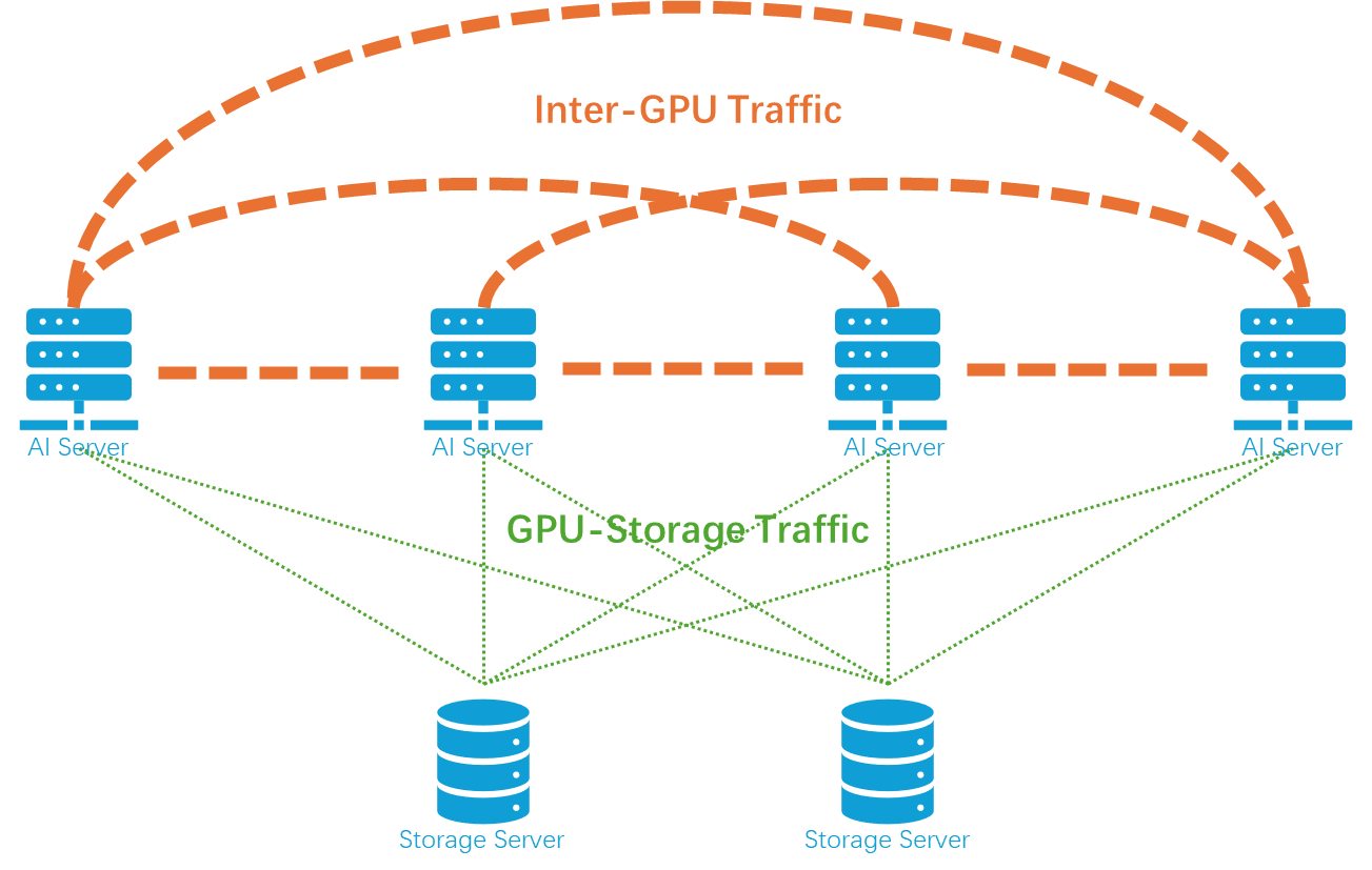
Figure 2. Network traffic categories during AI training
Among them, the network traffic within an AI data center is very different from the traffic within a traditional data center. It has the characteristics of broadcast, ultra-large traffic, ultra-low latency, ultra-high frequency, zero tolerance for packet loss, and strict time synchronization. This is closely related to the training method of large AI models. To handle large datasets and model parameters, several parallel training techniques are employed:
- Data Parallelism: Different sample data are fed to different GPUs to speed up training. This is similar to teachers grading assignments. The students’ assignments are distributed among multiple teachers for grading, thereby speeding up the process.
- Tensor Parallelism: The model’s parameter matrix is divided into sub-matrices distributed across GPUs, addressing memory limitations and accelerating computations. Still using grading assignments as an example, a student’s assignments in different subjects are distributed to different teachers for grading simultaneously, thereby speeding up the grading process for each student’s assignments.
- Pipeline Parallelism: The model is divided into stages, with each stage assigned to different GPUs, improving memory utilization and resource efficiency. Still using grading assignments as an example, different parts of the same test are graded by different teachers. After one part is graded, it is passed on to the next teacher. Although the grading time for each individual assignment does not shorten, this method increases the overall grading speed on a larger scale.
- Mixture of Experts (MoE) Parallelism: Multiple expert models are combined, and different experts are assigned to different GPUs. Dynamic selection of experts for different inputs reduces computation and addresses memory limitations. This is similar to a hospital that consists of multiple specialized departments, with a reception desk responsible for directing patients to the appropriate departments.
The three technologies of data parallelism, tensor parallelism, and pipeline parallelism are usually used in combination, known as 3D parallelism. In this approach, GPUs are organized into a cluster according to these three dimensions, as shown in the Figure 3.
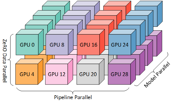
Figure 3. 3D parallel GPU cluster[7]
Taking Llama3-70B training as an example, a GPU cluster with 8-way tensor parallelism, 8-way pipeline parallelism and 16-way data parallelism, totaling 1024 blocks, can be used. Tensor parallelism is generally used within a single host, while data parallelism and pipeline parallelism are used between hosts.
In these three dimensions, the traffic patterns between GPUs differ significantly from one another.
Parallel Training Generates Most Network Traffic in AI Data Centers
Data Parallel Training Network Traffic Analysis
In data parallelism, the main network traffic arises from gradient synchronization, which occurs after processing each mini-batch. This synchronization is implemented through an all-reduce operation. In a cluster consisting of G × GPUs, ideally, all GPUs are fully connected. Each GPU sends data to the other
(G−1) × GPUs separately, requiring a total of G × (G−1) data flows, as shown in the Figure 4. Due to cost constraints, topologies such as ring networks and fat trees can be used to achieve logical full connectivity, but these topologies introduce additional transmission delays.
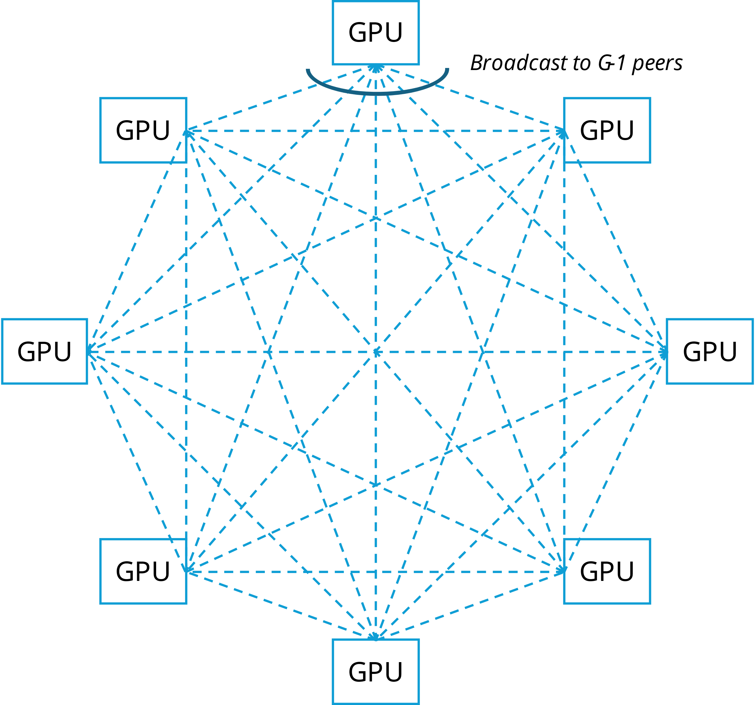
Figure 4. Data parallel gradient synchronization all-reduce traffic diagram
Assumptions:
- P is the number of model parameters. Since the gradient size is the same as the parameter size, it is the number of gradients. It uses the BFLOAT16 data format, and each parameter occupies 2 bytes.
- G is the number of GPUs, and the size of the gradient calculated by each GPU is 2P bytes.
- B is the batch size, D is the total number of samples in the dataset, and the number of mini-batches in each epoch is N = D/B .
The total network traffic (the sum of all GPUs’ sends and receives) can be calculated using the following formula:
Network traffic for each mini-batch:
2 × P × G × (G-1)
Network traffic per epoch:
2 × N × P × G × (G-1)
Take the Llama3 70B model as an example to calculate:
Assume that the number of model parameters P = 70 billion. The number of samples in the C4 dataset is 364.6 million, and the batch size is 2048. Each epoch contains about 178,000 mini-batches. 8 GPUs are used for data parallelism.
Network traffic per mini-batch:
2 × P × G × (G-1) = 2 × 70B × 8 × (8-1) = 7,840GB
Total network traffic per epoch:
2 × N × P × G × (G-1) = 2 × 178000 × 70B × 8 × (8-1) ≅ 1,396PB
FSDP Training Network Traffic Analysis
FSDP (Fully Sharded Data Parallel)[8] is an improved data parallel technology. It incorporates the advantages of tensor parallelism into data parallelism by sharding model parameters across multiple GPUs, achieving more efficient memory utilization and communication. The main features of FSDP include:
- Parameter sharding:
The parameters of the model are stored in slices among G × GPUs, and each GPU only stores of the 1/G parameters.
During forward propagation, the required parameter fragments are dynamically loaded into memory and released after calculation.
- Gradient sharding and synchronization:
Similar to data parallelism, FSDP also needs to synchronize gradients, but it only synchronizes the gradients of shards, reducing communication overhead.
- Layer-wise Sharding:
FSDP usually performs parameter sharding and calculation in layers, which further reduces the memory burden of a single GPU. The parameters of each layer are gathered on the required GPU during calculation and are dispersed after the calculation is completed.
In FSDP, network traffic comes from parameter collection in the forward propagation and gradient synchronization in the backward propagation.
The parameter collection of the forward propagation is completed by the all-gather operation. The communication complexity of all-gather is the same as that of all-reduce.
- Assume that the total number of model parameters is P, the number of GPUs is G, and the number of mini-batches is N.
- Each GPU only stores P/G parameters, but the parameters of the entire model need to be collected during calculation.
Therefore, the number of bytes transferred in each all-gather operation is:
2 × P / G × G × (G – 1) = 2 × P × (G – 1)
The total network traffic in one epoch is:
2 × N × P × (G – 1)
Due to the layer-wise sharding, this traffic are divided into L transmissions, where L is the number of layers in the model.
The gradient synchronization of backward propagation is completed by the all-reduce operation. Since the parameters of each GPU are only 1/G of the original, the total network traffic in an epoch is only 1/G of the normal data parallel operation, that is,
2 × N × P × (G – 1)
Take the Llama3 70B model and C4 dataset as an example to calculate the total network traffic per epoch:
4 × N × P × (G – 1) = 4 × 178000 × 70B × (8 – 1) ≅ 349PB
Tensor Parallel Training Network Traffic Analysis
In tensor parallelism, model parameters are distributed to G GPUs, and each GPU only stores 1/G parameters. Network traffic mainly comes from the transmission of intermediate activations during the forward propagation and the synchronization of gradients during the backward propagation.
In the forward propagation, the intermediate activations calculated by each GPU need to be merged, which is completed by an all-reduce operation. For each token, merges are performed twice in each layer of the model, , resulting in a very high frequency.
- Assuming that the number of tokens in the dataset is T and the model has L layers, 2 × T × L intermediate activations will be merged in one epoch process.
- Assume that the hidden state size of the model is H, the number of GPUs is G, the data format is BFLOAT16, and the communication amount per all-reduce operation is 2 × H × G × (G – 1)
Therefore, during one epoch, the total network traffic of the intermediate activations is:
4 × T × L × H × G × (G – 1)
In the backward propagation, the gradients need to be synchronized between GPUs. This synchronization occurs twice during the processing of each layer, with all gradients being merged by an all-reduce operation. This synchronization occurs during the processing of each layer of each mini-batch. A total of 2 × N × L communications.
Assuming the total number of parameters is P, the total network traffic for gradient synchronization is:
4 × N × L × P × (G – 1)
Taking the Llama3 70B model and the C4 dataset as an example, the total number of tokens in the C4 dataset is about 156B [9].
Total network traffic per epoch:
4 × T × L × H × G × (G – 1) + 4 × N × L × P × (G – 1)
= 4 × 156B × 80 × 8192 × 8 × (8 – 1) + 4 × 178000 × 80 × 70B × (8 – 1)
= 22,900,899,840GB + 27,915,731,200GB ≅ 50,816PB
Pipeline parallel Training Network Traffic Analysis
In pipeline parallelism, network traffic mainly comes from the transfer of intermediate activations in the forward and backward propagations. Unlike tensor parallelism, the transfer of these flows occurs between the front and back stages of the model, does not require all-reduce operations, and the frequency is greatly reduced.
During the forward propagation, the intermediate activations of each stage need to be transferred to the GPU where the next stage is located.
Assuming there are G stages (that is, G GPUs), the dataset has T tokens, the hidden state size is H, and the data format is BFLOAT16, then in one epoch, the total network traffic of the intermediate activation is:
2 × T × H × (G – 1)
During the backward propagation, the intermediate activations of each stage need to be sent back to the GPU where the previous stage is located to calculate the gradient of the previous stage.
Assuming the total number of parameters is P, the total network traffic of the intermediate activations of backward propagation is:
2 × T × H × (G – 1)
Taking the Llama3 70B model as an example, the total network traffic per epoch is calculated as follows:
4 × T × H × (G – 1) = 8× 156B × 8192 × (8 – 1) ≅ 35.8PB
Comparative Analysis of Data/Tensor/Pipeline Parallel Training Network Traffic
In summary, among the three parallel methods, the network traffic of tensor parallelism is the largest and the frequency is the highest, the traffic of pipeline parallelism is the lowest, and the communication frequency of data parallelism is the lowest. As shown in the following table, in each epoch process:
| Traffic patterns | Total network traffic in the backward propagation | Backward communication times | Total network traffic in the forward propagation | Forward communication times | |
| Data Parallelism | all-reduce | 2 × N × P × G × (G-1) | 1 | 0 | 0 |
| FSDP | all-gather + all-reduce | 2 × N × P × (G-1) | L | 2 × N × P × (G-1) | L |
| Tensor Parallelism | all-reduce | 4 × N × P × L × (G-1) | 2 × L | 4 × L × T × H × (G-1) × G | 2 × L × T |
| Pipeline Parallelism | Point-to-point | 2 × T × H × (G-1) | G-1 | 2 × T × H × (G-1) | G-1 |
Where P is the model parameter, T is the number of tokens, L is the number of model layers, H is the hidden state size, G is the number of GPUs, and N is the number of mini-batches.
3D Parallel Training Network Traffic Analysis
3D parallelism is a method that combines data parallelism, tensor parallelism, and pipeline parallelism to further improve the efficiency and scalability of training LLMs. Assuming that there are Gtp × Gpp × Gdp GPUs forming a 3D parallel array, all P parameters will be divided into Gtp × Gpp parts, each of which is P/ Gtp / Gpp. There is network traffic in the three dimensions of model parallelism, pipeline parallelism, and data parallelism, as shown in Figure 5.
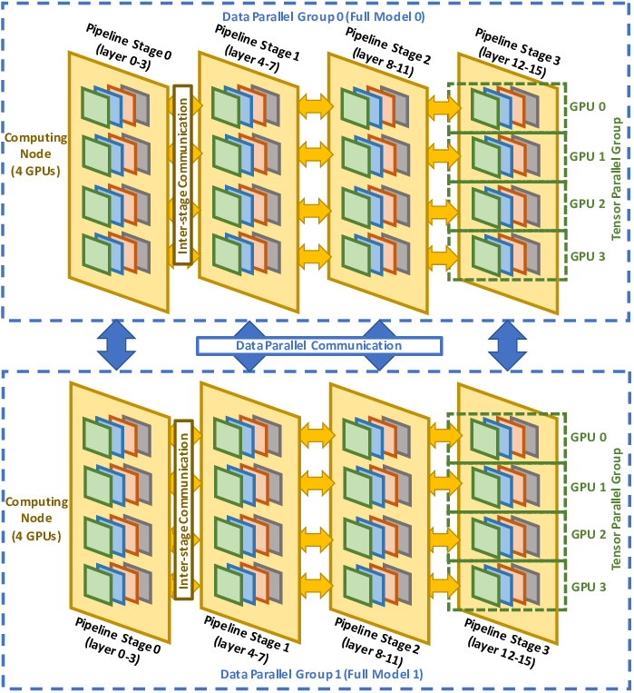
Figure 5. 3D parallel network traffic diagram[10]
Gradient synchronization is performed during backward propagation, which is divided into:
- Gradient synchronization on the tensor dimension is performed in each layer of the model and each group of the data dimension, a total of L × Gdp times.
- Gradient synchronization on the data dimension is performed in each stage of the pipeline dimension and each group of the tensor dimension, a total of Gtp × Gpp times.
As shown in Figure 6.
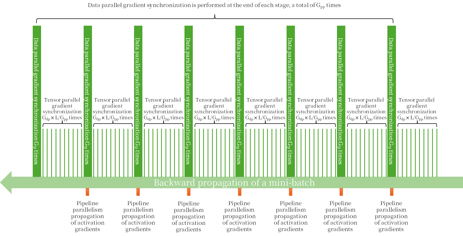
Figure 6. 3D parallel backward propagation network traffic diagram
Thus, in one epoch, the total network traffic for gradient synchronization is:
4 × N × P/Gtp /Gpp × Gtp × (Gtp – 1) × L × Gdp + 2 × N × P/Gtp /Gpp × Gdp × (Gdp – 1) × Gtp × Gpp
= 2 × N × P × Gdp × [2 × L × (Gtp – 1) / Gpp + (Gdp – 1)]
In addition, during the backward propagation, the intermediate activations are passed in the pipeline parallel dimension, and the traffic is:
2 × T × H × (Gpp – 1)
Therefore, in one epoch, the total traffic of the entire backward propagation is:
2 × N × P × Gdp × [2 × L × (Gtp – 1) / Gpp + (Gdp – 1)] + 2 × T × H × (Gpp – 1)
In the forward propagation, the transfer of intermediate activations is performed alternately in tensor parallelism and pipeline parallelism, where the tensor parallel activation transfer contains 2 all-reduce operations each time, as shown in Figure 7.
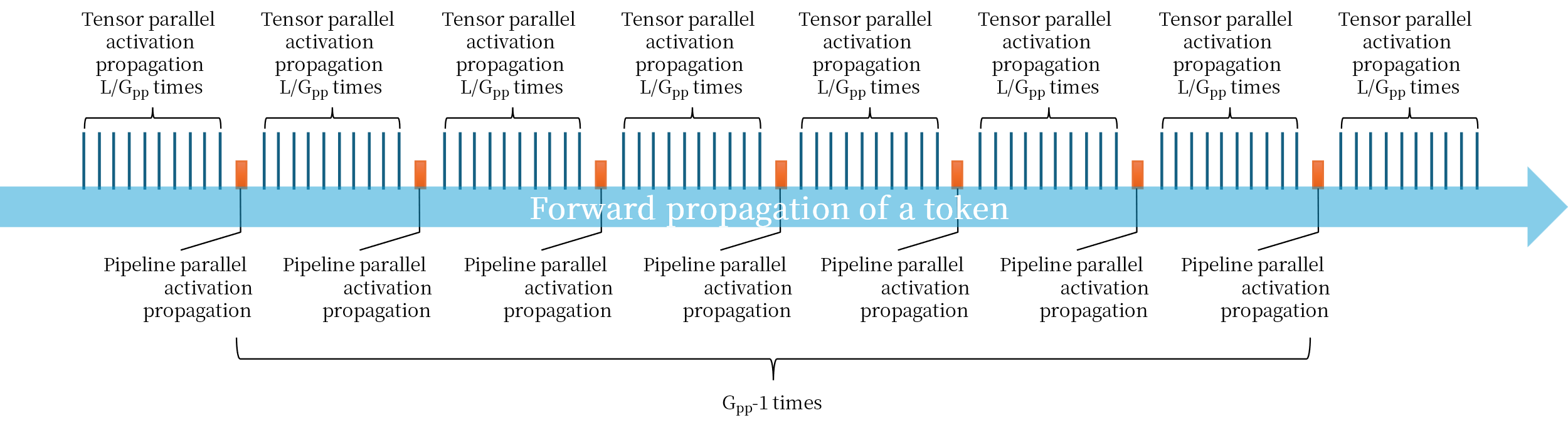
Figure 7. 3D parallel forward propagation network traffic diagram
Therefore, in one epoch, the total network traffic for forward propagation is:
4 × T × H × L × Gtp × (Gtp – 1) + 2 × T × H × (Gpp – 1)
Using the Llama3-70B model, 8-way tensor parallelism, 8-way pipeline parallelism and 16-way data parallelism, a total of 1024 GPUs are used for training, and the total traffic generated by one epoch is about 85EB. This is equivalent to the total traffic of the entire Internet for 2.5 days[11]. If a switch with a capacity of 51.2T is used, it will take about 20 days to complete the transmission if it runs at full capacity 24 hours. Considering that one pre-training usually contains about 100 epochs, if the training needs to be completed in 100 days, at least 20 switches of 51.2T are needed to transmit the data generated during the training process.
Unveiling Network Traffic for AI Inference
AI Parallel Inference Network Traffic Analysis
The AI inference program first loads the model into the GPU memory and then waits for input for inference. Unlike the training process, the inference process only has forward propagation.
When performing inference with a LLM, even though the model is often compressed, such as through 4-bit quantization, the model size may still exceed the memory capacity of a single GPU. At this time, tensor parallelism is needed. Even if a single GPU can accommodate the entire model, tensor parallelism can speed up the inference process. If the number of concurrent users is large and a single GPU cannot respond in time, data parallelism is required.
The inference process of LLMs can be divided into two steps: the Prefill step and the Decode step:
- Prefill Step: This step generates an input token sequence based on the prompt input by the user, batches these tokens, calculates the KV (Key, Value) cache, and generates the first output token. This step can be considered as the LLM understanding the user input. The KV cache stores the context information of the input sequence. This step is characterized by the need for a large amount of calculation.
- Decode Step: This step is a recursive process that calculates the next token based on the previously generated token sequence and KV cache until the complete output is generated. This step can be considered as the LLM speaking word by word, which requires high-speed memory access and low computational effort.
Since the two steps have different requirements for GPUs, the Prefill-Decode disaggregation can be used, with two different types of GPUs taking on the computing tasks of the Prefill and Decode steps respectively and executing them sequentially. In this case, the KV cache needs to be transferred between the two steps.
When deploying in a production environment, the above methods are usually combined[12]. As shown in Figure 8:
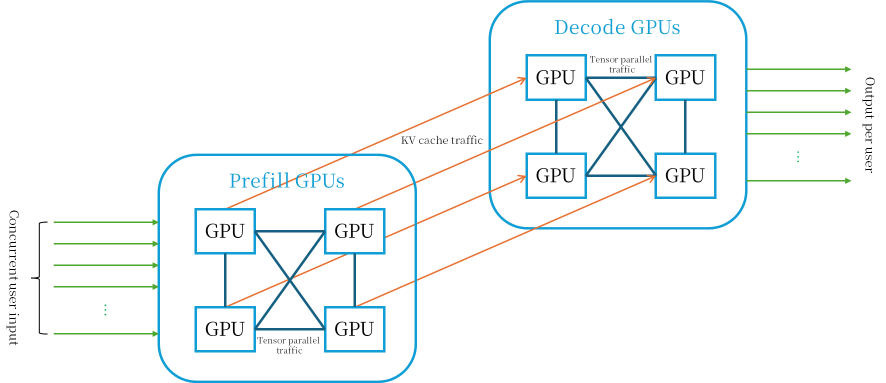
Figure 8. AI parallel inference GPU cluster
Assume that the number of concurrent users is U, the data parallel dimension is Gdp, the tensor parallel dimension is Gtp, the average length of the user prompt is Sin tokens, and the average length of the generated output is Sout tokens.
When tensors are parallelized, forward propagation generates network traffic between GPUs, and the intermediate activations calculated by each GPU need to be merged, which is completed by the all-reduce operation.
Assume that the model has L layers. In one inference process, in the Prefill step, Sin input tokens are batch merged twice in each layer of the model, for a total of 2 × L times. And in the Decode step, for each output Token, it is merged twice in each layer of the model, for a total of 2 × Sout × L times. As shown in Figure 9.
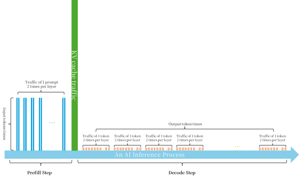
Figure 9. AI parallel inference network traffic diagram
Assume that the hidden state size of the model is H, the number of GPUs is G, the data format used for calculating activation is FLOAT16, and the network traffic per all-reduce is:
2 × H × Gtp × (Gtp – 1)
In the Prefill step, all Sin input tokens are batch merged twice in each layer of the model, a total of 2 × L times. In the Decode step, for each token, it is merged twice in each layer of the model, a total of 2 × Sout ×L times.
Therefore, for U users’ concurrent inference, the total network traffic of the intermediate activations is:
4 × U × (Sin + Sout) × L × H × Gtp × (Gtp – 1)
In addition, in one inference, the size of the KV cache is:
4 × Sin × L × H
Therefore, for U users’ concurrent reasoning, the network traffic transmitted by KV cache is:
4 × U × Sin × L × H
Take the Llama3-120B model as an example. The model has 140 layers, the hidden state size is 8192, the tensor parallelism is 4, the average length of the user prompt is Sin, which is 256 tokens, and the average length of the generated output is Sout, which is 4096 tokens. The inference traffic required to support 100 concurrent user requests is:
4 × 100 × (256 + 4096) × 140 × 8192 × 4 × (4 – 1) + 4 × 100 × 256 × 140 × 8192= 21.896TB
The traffic transmitted by the KV cache is not large, about 1.17 GB per user, but it needs to be transmitted once in about 10 ms. If it is transmitted using one 800G port, the fastest time is 11.7 ms.
What is the Difference Between Network Traffic for AI Training and AI Inference?
Although this traffic is much smaller than the network traffic during training, it is worth noting that inference needs to be completed in a very short time. Assuming that the inference speed is at least 100 tokens/s and the parallel acceleration ratio is 90%, the inference speed of each token should be less than 1ms, and KV caching needs to be completed in about 10ms. The entire network throughput should be greater than
4 × 100 × 140 × 8192 × 4× (4- 1) / 0.001 + 4 × 100 × 140 × 8192 /0.01 = 5551GB/s ≅ 44.4Tbps
In other words, a switch with a capacity of 51.2T can support the inference of up to 115 concurrent users.
Unveiling Network Traffic for AI Data Storage
Dataset Loading Network Traffic Analysis
In one epoch, the entire training set is traversed once, and if evaluation is performed, the validation set is also traversed once. The following assumes that evaluation is performed in each epoch and the storage size of the entire dataset is D.
- In data parallelism, the entire dataset is read from the storage servers and loaded onto different GPUs through scatter operations. The total network traffic is D.
- When tensors are parallelized, the entire dataset is read from storage servers and sent to all GPUs through broadcast operations. The total network traffic is D × G.
- When the pipeline is parallel, the entire dataset is read from the storage servers and fed to the first GPU in the pipeline, with a total network traffic of D .
- In 3D parallelism, the entire dataset is read from the storage servers, distributed in the data parallel dimension, and broadcast in the tensor parallel dimension. The total network traffic is D × Gtp.
Taking the C4 dataset as an example, the size of the dataset is about 38.5 TB. Assuming that the number of tensor parallel GPUs is 8, the network traffic generated by loading the dataset in each epoch in 3D parallelism is 308TB.
Checkpoint Storage Network Traffic Analysis
Checkpoint stores model parameters, optimizer status, and other training status (including model configuration, training hyperparameters, log information, etc.). The optimizer includes gradient, momentum, and second-order moment estimation, etc. The size of each data type is equal to the model parameter. The size of other training status can be ignored. Assuming the model parameter is P, the data format is BFLOAT16, and the optimizer is Adam/ AdamW, the total checkpoint size is:
2 × P + 2 × P × 3 = 8 × P
This checkpoint needs to be saved in the storage servers. Although in tensor parallelism, pipeline parallelism, and 3D parallelism, these data are gathered from multiple GPUs to the storage servers through the gather operation, the total amount of data is a checkpoint size anyway. Assume that each epoch is stored once. In this way, the traffic generated by each epoch is:
8 × P
Taking the Llama3-70B model as an example, assuming that each epoch is stored, the generated storage traffic is 560GB.
Conclusion: AI Data Center Network Traffic has Unprecedented Characteristics
From the previous analysis, we can see that the network traffic generated by LLMs in AI data centers has the following unprecedented characteristics:
- Ultra-high bandwidth: One epoch generates 85EB of data, which is equivalent to the traffic of the entire Internet for 2.5 days.
- Ultra-low latency: The processing of a training sample will generate more than 100GB of data, which needs to be transmitted in less than 1 millisecond, which is equivalent to the transmission speed of 1,000 × 800G interfaces.
- Ultra-high frequency: During the processing of a single inference, each token generates 2 traffics at each layer. To achieve an inference speed of 100 tokens per second, more than 28,000 communications per second are required.
- All-reduce and all-gather operations between GPU servers bring broadcast traffic, which is synchronized between tens of thousands of GPUs, that is, hundreds of millions of GPU-GPU pairs.
- Zero tolerance for packet loss: Based on the barrel principle, during collective communication, packet loss and retransmission of traffic between just one pair of GPUs will cause a delay in the entire collective communication, causing a large number of GPUs to enter idle waiting time.
- Strict time synchronization: Both training and Inference traffic follow very strict periodical rules. Also based on the barrel principle, if the GPU clocks are not synchronized, the same amount of calculation will take different times, and the faster GPU will have to wait for the slower GPU.
Asterfusion CX864E-N 800G Ultra Ethernet Switch is born for AI Data Center Traffic

This traffic pattern has triggered the upgrade of data center switches. The Asterfusion CX864E-N 800G switch is just such an Ultra Ethernet Switch. It has the following features:
- Ultra-large capacity, supporting 64 x 800G Ethernet ports and a total switching capacity of 51.2T.
- Ultra-low latency switching network, achieving the industry’s strongest 560ns cut-through latency on 800G ports.
- 200+ MB large-capacity and high-speed on-chip packet cache significantly reduces the storage and forwarding latency of RoCE traffic during collective communications.
- Intel Xeon CPU + large-capacity expandable memory, running the continuously evolving enterprise SONiC – AsterNOS network operating system, and directly accessing the packet cache through DMA to process network traffic in real time.
- INNOFLEX programmable forwarding engine can adjust the forwarding process in real time according to business needs and network status, minimizing packet loss caused by network congestion and failure.
- FLASHLIGHT refined traffic analysis engine measures the delay and round-trip time of each packet in real time, and implements adaptive routing and congestion control through intelligent analysis by the CPU.
- 10 nanosecond PTP/SyncE time synchronization ensures synchronous computing of all GPUs.
- Open API, open all functions to the AI data center management system through REST API, collaborate with computing devices, and realize automatic deployment of GPU clusters.
Embrace the Future of AI Data Center Network Infrastructure with Asterfusion
Visit:https://cloudswit.ch/blogs/future-of-ai-data-center-network-infrastructure/
In short, the Asterfusion CX864E-N 800G switch not only maintains extreme performance but also achieves programmability and upgradeability. It synergizes with computing devices to create 100,000-level GPU cluster interconnections, transforming the data center into an AI super factory comparable to supercomputers.
- https://the-decoder.com/gpt-4-architecture-datasets-costs-and-more-leaked/ ↑
- https://commoncrawl.github.io/cc-crawl-statistics/ ↑
- https://www.tensorflow.org/datasets/catalog/c4 ↑
- https://developer.nvidia.com/blog/scaling-language-model-training-to-a-trillion-parameters-using-megatron ↑
- https://www.microsoft.com/en-us/research/blog/deepspeed-extreme-scale-model-training-for-everyone/ ↑
- https://pytorch.org/tutorials/intermediate/FSDP_adavnced_tutorial.html?highlight=fsdp ↑
- https://ar5iv.labs.arxiv.org/html/2104.08758v1 ↑
- https://www.sandvine.com/blog/sandvines-2024-global-internet-phenomena-report-global-internet-usage-continues-to-grow ↑
- https://www.linkedin.com/pulse/optimizing-inference-large-language-models-strategies-ravi-naarla-d6ppc/


